Why Probability Theory is important while studying Machine Learning?

• Machine Learning is all about finding the pattern exhibited by the data.
• Machine Learning tells that the observations are noisy instances of much simpler rule. To learn that rule from the data, is the job of Machine Learning algorithm.
• As the rules/patterns exhibited by the data are not explicit, hence there is some degree of uncertainty associated with the “learned rule” from the data.
• Probability theory is the mathematical framework to deal with uncertainties.
• Hence, Probability theory is the indispensable tool to study machine learning.

What is Probability?

Probability is a mathematical description of randomness and uncertainty. It is a way to measure or quantify uncertainty. Another way to think about probability is that it is the official name for “chance.”

Probability is the Likelihood of Something Happening.

One way to think of probability is that it is the likelihood that something will occur.

Probability is used to answer the following types of questions:

• What is the chance that it will rain tomorrow?
• Chance that a stock will go up in price.
• What is the probability that I will win the lottery?

Each of these examples has some uncertainty. For some, the chances are quite good, so the probability would be quite high. For others, the chances are not very good, so the probability is quite low.

Few Notions:

• A Random Experiment is a process whose all possible outcomes are known, but which outcome will occur at a certain trial is unknown until the experiment is performed.
• Sample Space of a Random Experiment is the collection of all possible outcomes of that experiment.
• An Event is the subset of the sample space which describes some possible outcomes of a random experiment.

Example: Rolling a dice is a Random Experiment. Whose Sample Space is {1, 2, 3, 4, 5, 6} and an Event could be “Obtaining an even number as outcome”.  

Notation: If ‘A’ be an event then P(A) denotes the probability of that event. The “probability” of an event tells us how likely it is that the event will occur.

Probability as Relative Frequency:

To estimate the probability of event A, written P(A), we may repeat the random experiment many times and count the number of times event A occurs. Then P(A) is estimated by the ratio of the number of times A occurs to the number of repetitions, which is called the relative frequency of event A.

To estimate the probability of event A, written P(A), we may repeat the random experiment many times and count the number of times event A occurs. Then P(A) is estimated by the ratio of the number of times A occurs to the number of repetitions, which is called the relative frequency of event A.

Relative Frequency of Event A= (Number of times A occurred)/ (Total number of repetitions)

Law of Large Numbers: The actual (or true) probability of an event (A) is estimated by the relative frequency with which the event occurs in a long series of trials.

What is the probability that the number rolled is even, when an ordinary fair die is rolled once? We’ll denote this event by E (for even). So, we are interested in finding P(E). Let’s analyze this problem:

• The random experiment is rolling a fair die once.
• The sample space of all possible outcomes in this case this is S = {1, 2, 3, 4, 5, 6}.
• The sample space of all possible outcomes in this case this is S = {1, 2, 3, 4, 5, 6}.
• We are interested in a particular type of outcome, which is represented by event E – getting an even number.
• Since 3 out of the 6 equally likely outcomes make up the event E (the outcomes {2, 4, 6}). Hence, P(E) = 3/6 = 0.5

Basic Rules of Probability

• 0 ≤ P(A) ≤ 1, Here A is an event. This is also known as range rule.
• P(S) = 1, Here S is the sample space. The sum of the probabilities of all possible outcomes is 1.
• P(Ac) = 1 – P(A), Here Ac=SA, called the complement of A.
• P(A∪B) = P(A) + P(B) – P(A∩B), This is called addition rule of probability. If A and B are disjoint event (i.e., A∩B=∅) then, P(A∪B) = P(A) + P(B)
• P(A∩B) = P(A) × P(B), If A and B are independent.
• P(A∪B∪C) = P(A) + P(B) + P(C) – P(A∩B)–P(B ∩C)– P(A∩C) + P(A∩B∩C)

Conditional Probability:

P(A|B), called Probability of Event ‘A’ given ‘B’ = (P(A∩B))/(P(B))

Example: Consider the following table which describes the smoking habit of  few persons.

Gender	Smoker	Not Smoker	Total
Male	187	53	240
Female	57	203	260
Total	244	256	500

• Let ‘M’ denotes the event of being ‘Male’, while ‘A’ represents the event of being ‘Smoker’.
• What is the conditional probability that a randomly chosen student is smoker, given that this student is female?

P(Smoker | Female)=  (P(Smoker and Female))/(P(Female))=  (57⁄500)/(260⁄500)=  57/260=0.2192

-This is known as multiplication rule of probability.

Law of total probability:

The total probability rule (also called the Law of Total Probability) breaks up probability calculations into distinct parts. It’s used to find the probability of an event, A, when you don’t know enough about A’s probabilities to calculate it directly. Instead, you take a related event, B, and use that to calculate the probability for A.

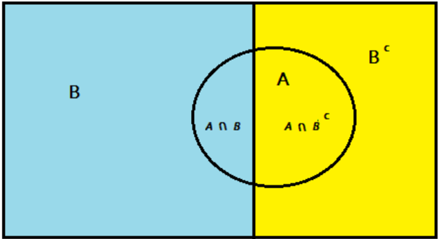
Thus, the total probability rule in this case is:

P(A)=P(A∩B)+P (A∩Bc)

P(A)=P(B)×P(A|B)+P(Bc )×P(A|Bc)

Example: 80% of people attend their primary care physician regularly; 35% of those people have no health problems crop up during the following year. Out of the 20% of people who don’t see their doctor regularly, only 5% have no health issues during the following year. What is the probability a random person will have no health problems in the following year?

Let us consider, here the event of person having no health problem is denoted by A and people seeing doctor is denoted by B.

• Then by theorem of total probability, P(A)=P(A∩B)+P (A∩Bc ).
• Then by multiplication rule of probability, P(A)=P(B)×P(A│B)+P(Bc )×P(A|Bc)
• P(A)=0.8×0.35+(1 -0.8)×0.05=0.28+0.01=0.29

Law of total probability for multiple events:

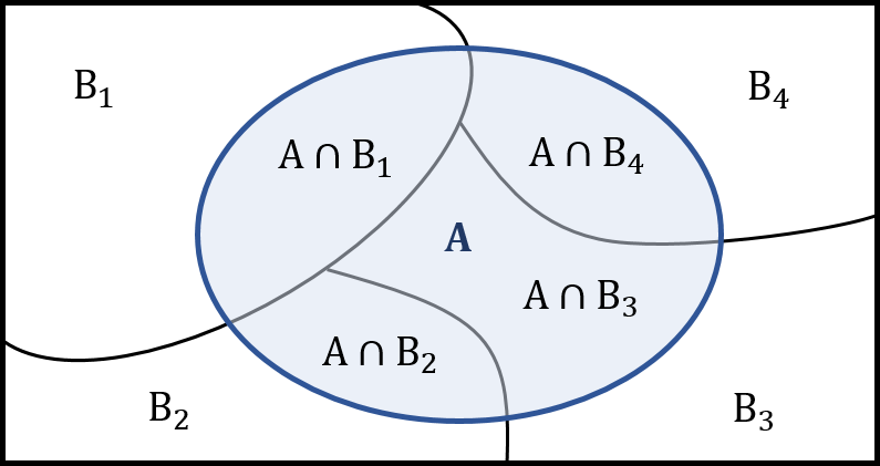
For n many events B1, B2, …, Bn

P(A)=P(A∩B1 )+P(A∩B2 )+ …+P (A∩Bn )

P(A) = ∑ P(A∩Bi ) ; [where i = 1 to n]

P(A) = ∑ P(A∩Bi ) = ∑ (P(Bi )×P(A|Bi)) ; [where i = 1 to n]

Bayes Rule:

From multiplication rule of probability: P(B)×P(A│B)=P (A∩B)= P(A)×P(B|A)

∴P(B│A)=  (P(A|B))/(P(A))×P(B)  , assuming that P(A)≠0

• Here P(B) is called the prior probability of B or initial degree of belief in the event B.
• Here P(B|A) is called the posterior probability of B or degree of belief in the event B after accounting for event A.
• The quotient (P(A|B))/(P(A)) is the support that event A provides for event B.

Example: Three machines produce the entire output of a Factory. The three machines account for 20%, 30%, and 50% of the factory output. The fraction of defective items produced is 5% for the first machine; 3% for the second machine; and 1% for the third machine. If an item is chosen at random from the total output and is found to be defective, what is the probability that it was produced by the third machine?

Let Xi denote the event that a randomly chosen item was made by the i th machine (for i = A, B, C). Let Y denote the event that a randomly chosen item is defective. Then P(XA )=0.2, P(XB )=0.3 and P(XC)=0.5

If the item was made by the first machine, then the probability that it is defective is 0.05; that is, P(Y | XA) = 0.05. Overall, we have P(Y|XA )=0.05, P(Y|XB )=0.03 and P(Y|XC)=0.01

What is the probability that the randomly chosen item is defective?

P(Y)= ∑ [P(Xi )×P(Y|Xi)] = 0.2×0.05+0.3×0.03+0.5×0.01=0.024 ; [where i = 1 to 3]

Hence around 2.4% of the total output of the factory is defective.

We are given that Y has occurred, and we want to calculate the conditional probability of XC. By Bayes’ theorem,

P(XC│Y)=  (P(Y|XC))/(P(Y))×P(XC )=  0.01/0.024×0.5=  5/24